Next: A Wavelet Parallel Code for Structure Detection
Up: Astrostatistics and Databases
Previous: A Multidimensional Binary Search Tree for Star Catalog Correlations
Table of Contents -- Index -- PS reprint -- PDF reprint
V.L.Oknyanskij
Sternberg Astronomical Ins., Universitetskij Prospekt 13, Moscow,
119899, Russia
Here we use Monte-Carlo simulations to estimate the significance of the
results. We estimate (with the 95% confidence level) that the probability
of getting the same result by chance (if the real V value was
equal to 0 days/year) is less then 5%. We also show that the method
can also determine the actual rate of increase
![]() of the time delay in artificial light curves,
which have the same data spacing, power spectrum and noise level as real ones.
of the time delay in artificial light curves,
which have the same data spacing, power spectrum and noise level as real ones.
We briefly consider some other possible fields for using the method.
At the previous ADASS Conference (Oknyanskij, 1997a, see also
Oknyanskij 1997b) we considered and used a new algorithm for
time-delay investigations in the case
when the time delay was a linear function of time and the
echo response intensity was a power-law function of the time delay.
We applied this method to investigate optical-to-radio delay in
the double quasar 0957+561 (generally accepted to be a case
of gravitational lensing). It was found in this way that the
radio variations (5 MHz) followed the optical ones, but that the
time delay was a linear function
of time with the mean value being about 2370 days and with the rate
of increase ![]() days/year.
days/year.
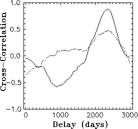
The cross-correlation function for this best fit is shown in Figure 1 together with the cross-correlation function for the data without any corrections for possible variability of the time delay value. The maximum of the cross-correlation for the last case (if V = 0 days/year) is less then 0.5. So we can note that our fit explains the real data significantly better then the simple model with some constant time delay. Meanwhile Monte-Carlo simulations are needed to estimate the significance of our result. The methodology of these estimations is briefly explained below.
 |
The idea of our Monte-Carlo test is the following:
1. We produce m=500 pairs of the simulated light curves which have
the same power spectra, time spacing, signal/noise ratio as the real optical and radio
data, but with constant value of time delay (![]() = 2370 days) and about
the same maximum values of cross-correlation functions.
= 2370 days) and about
the same maximum values of cross-correlation functions.
2. We apply the same method and make all the steps the same as was done
for the
real data (Oknyanskij, 1997a,b), but for each of m pairs of the
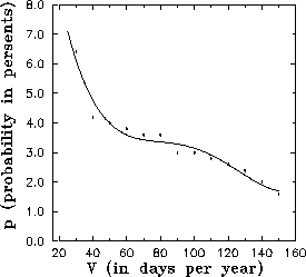
simulated light curves. The proportion p(V) of obtained ![]() (see Figure 2) that yield a value bigger or equal to V provides
an estimate of the
(see Figure 2) that yield a value bigger or equal to V provides
an estimate of the ![]() value. When
value. When ![]() ,standard error of the estimated
,standard error of the estimated
![]() value can be approximated by well-known formula
value can be approximated by well-known formula
![]() (see Robbins and Van Ryzin 1975).
An approximate 95% confidence interval for the true p value can be written as
(see Robbins and Van Ryzin 1975).
An approximate 95% confidence interval for the true p value can be written as
![]() . As it is seen from Figure 2 -
. As it is seen from Figure 2 - ![]() . The approximate standard error of this value is about
. The approximate standard error of this value is about ![]() .We can write the 95% confidence interval for
.We can write the 95% confidence interval for ![]() and conclude with a 95% confidence level that
and conclude with a 95% confidence level that ![]() 5%.
So the H0 can be rejected, i.e., time delay is some increasing function of time.
For the first step we assume that it is a linear function of time and
found V = 110 days/year, a value approximately equal to the true one.
5%.
So the H0 can be rejected, i.e., time delay is some increasing function of time.
For the first step we assume that it is a linear function of time and
found V = 110 days/year, a value approximately equal to the true one.
3. To show that the method has real abilities to determinate a value of
of the time delay rate of increase in the light curves we again use
Monte-Carlo simulation as it is explained in (1) and (2), but the actual
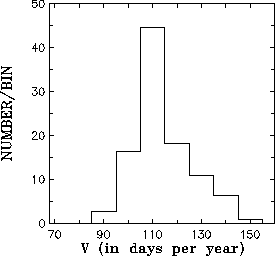
![]() value is 110 days/year. Then we obtain the histogram
(Figure 3), which shows the distribution of obtained
value is 110 days/year. Then we obtain the histogram
(Figure 3), which shows the distribution of obtained ![]() values.
It is clear that the distribution has some asymmetry, which could be a reason
for some small overestimation of V value, since the mathematical
expectation of mean
values.
It is clear that the distribution has some asymmetry, which could be a reason
for some small overestimation of V value, since the mathematical
expectation of mean ![]() ' is about 114 days/year.
Meanwhile we should note that the obtained histogram shows us the ability of
the method to get the approximate estimate of the actual
' is about 114 days/year.
Meanwhile we should note that the obtained histogram shows us the ability of
the method to get the approximate estimate of the actual ![]() value,
since the distribution in the Figure 3 is quite narrow.
Using this histogram we approximately estimate the standard error
value,
since the distribution in the Figure 3 is quite narrow.
Using this histogram we approximately estimate the standard error
![]() 15 days/year (for V value, which has been
found for Q 0956+561).
15 days/year (for V value, which has been
found for Q 0956+561).
 |
 |
We have found a time delay between the radio and optical flux
variations of Q 0957+561 using a new method (Oknyanskij, 1997a,b),
which also allowed us to investigate the possibilities
that (1) there is some change of time delay that is a linear function of time,
and (2) the radio response function has power-law dependence on the time
delay value. Here we estimate the statistical significance of the result and
the ability of the method to find the actual value of V as well as its
accuracy. We show that with 95![]() confidence level
the probability of getting a value of
confidence level
the probability of getting a value of ![]() 110 days/year (if actual
110 days/year (if actual
![]() would be equal to 0 days/year) is less then 5
would be equal to 0 days/year) is less then 5![]() . We estimate that standard error of the V value (which has been found
for Q 0957+561) is about 15 days/year.
. We estimate that standard error of the V value (which has been found
for Q 0957+561) is about 15 days/year.
Finally, we can briefly note some other fields where the method may be used:
1. Time delay between continuum and line variability in AGNs may be a function of time as well as the response function possibly being some function of time. So our method can be useful for this case.
2. Recently, it has been suggested by Fernandes et. al (1997) that variability of different AGNs might have coincident recurrent patterns in their light curves. However it has been found that the time-scales for these patterns in NGC 4151 and 5548 are about the same, there are a lot of reasons to expect that the patterns in AGN light curves may be similar, but have different time scales. It is possible to use our method with some enhancements to investigate this possibility. Some Monte-Carlo estimations of the significance would be also very useful. The probability that these common recurrent patterns in AGNs occur by chance should be estimated.
Fernandes, R.C., Terlevich R. & Aretxaga I. 1997, MNRAS, 289, 318
Oknyanskij, V.L., & Beskin, G.M. 1993, in: Gravitational Lenses in the Universe: Proceedings of the 31st Liege International Astrophysical Colloquium, eds. J.Surdej at al. (Liege, Belgium: Universite de Liege, Institut d'Astrophysique), 65
Oknyanskij, V.L. 1997a, in Astronomical Data Analysis Software and Systems VI, ASP Conf. Ser., Vol. 125, eds. Gareth Hunt and H. E. Payne (San Francisco, ASP), 162
Oknyanskij, V.L. 1997b, Ap&SS, 246, 299
Robbins, H. & Van Ruzin, J. 1975, Introduction to Statistic (Science Research Associates, Chicago), 167
Next: A Wavelet Parallel Code for Structure Detection
Up: Astrostatistics and Databases
Previous: A Multidimensional Binary Search Tree for Star Catalog Correlations
Table of Contents -- Index -- PS reprint -- PDF reprint