Table of Contents -- Index -- PS reprint -- PDF reprint

Astronomical Data Analysis Software and Systems VII
ASP Conference Series, Vol. 145, 1998
Editors: R. Albrecht, R. N. Hook and H. A. Bushouse

On the Need for Input Data Control in Pipeline Reductions

J.-P. De Cuyper and H. Hensberge
Royal Observatory of Belgium, Ringlaan 3, B-1180 Brussel, Belgium

 

Abstract:

An analysis of series of flat-field exposures obtained in echelle mode adds support to the view that the performance of an instrument should be monitored closely and described quantitatively. This simplifies enormously the data reduction procedure and allows the user to interpret high-quality data correctly.

       

1. Introduction

Nowadays it is not unusual for the knowledge about an instrument acquired by the design and construction team to be only partially transmitted to those developing the data reduction software or operating the instrument; the feedback to the observer is still smaller. This may result in confusion about basic instrumental parameters, the precision of the set-up, the amount and distribution of calibration frames which are required and finally the assumptions on which the data reduction procedure should rely. The data set then does not deliver the precision aimed at during observing, or observing time was spent inefficiently. The concept of pipeline reductions and on-line controlled operation of the instrument and of the observational procedure offer unprecedented possibilities for delivering data with known error characteristics, provided that the instrumental design, the set-up, the calibration and the data reduction procedure are tuned to each other at a consistent level of accuracy. Our experience with echelle spectroscopy indicates that, as a visiting astronomer, it is impossible to collect the information needed to obtain this goal. Moreover, it is not at all evident to what extent forthcoming pipelines will include realistic error estimates (in addition to random noise estimates).

2. An Example: Series of flat-fields

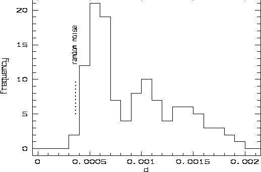
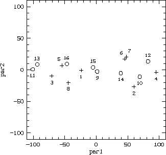
The results shown here refer to two adjacent series of eight consecutively taken flat-fields (tungsten lamp exposures). The telescope was in the zenith and tracking was off. The analysis method applied is insensitive to global changes in intensity and to small changes in location, width or shape of the cross-order profile (these changes are below 0.5% in intensity and within 0.02 pix for the other quantities in both series). For each pair of frames, a parameter d indicating the lack of similarity in the shape of the blaze profile was computed (Figure 1). It turns out that the excess of d over its value calculated from the case of random noise can be modelled as a ``distance'' between frames (Figure 2).

  

Figure 1: Histogram of the dissimilarity parameter d for all combinations of 2 out of the 16 flat-fields. d² scales with the variance due to long-range ($\approx$ 100 pixels) deformations in ratios of extracted flat-field orders, except for an offset due to the contribution of random noise. The value for pure random noise is indicated

  

Figure 2: The dissimilarity of flat-fields represented as an Euclidian distance between frames situated in a plane (par1, par2). The numbering indicates the order of the exposures. Notice the usually large distance between consecutive frames, and the similarity between the series 1-8 and 9-16

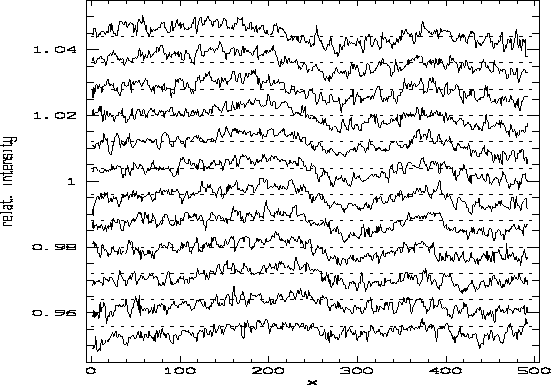
The lack of repeatability in subsequent frames is due to instabilities that grow and disappear, rather than to a slow, continuous change with time. Consecutively taken frames differ more than the ones separated by an intermediate frame, and the global pattern of changes repeats in the two independent series (Figure 2). Relative deformations in the shape of the blaze profile appear over several spectral orders in the same set of rows of the detector (see e.g., Figure 3 near $x \approx 300$).

It is not our intention to show that things can sometimes go very wrong, but merely that the accuracy is generally limited by systematic errors. The example shown above does not refer to an exceptional malfunctioning, but to a common situation. Notice that it is not uncommon to detect stronger effects when comparing exposures taken with longer time delays and/or in different telescope positions. The detectability of such systematic effects sets a natural limit on the precision of order merging (since the intensity ratio of the wavelength overlap region of consecutive orders is affected), on the level up to which faint, shallow spectral features can be trusted and on the precision of the continuum placement.

  

Figure 3: Relative deformation of the blaze profile expressed as the intensity ratio of the sum of frames #11 and #13 to the sum of #10 and #12. This ratio is shown along 12 consecutive orders, shifted vertically for clarity (the dashed lines indicate the relative intensity level 1.0 for each order). Instrument: CASPEC, detector: ESO CCD #32

3. Data Reduction Strategy

Experience with echelle spectroscopy confirms that the previous example is not an isolated case of bias. Systematic errors are detectable in almost all types of frames and they influence directly the applicability and the accuracy of the data reduction algorithms. Depending on the ratio of systematic to random noise, algorithms that are based on the dominance of random noise (such as the detection of radiation events, the application of optimal extraction and any reduction step involving non-robust least-squares fitting) may need refinements.

Rather than commenting on specific sources of bias, we like to outline a procedure, interconnecting the different phases from instrument development and testing to data reduction software development, that in our opinion would permit the user to evaluate properly the quality of the final data with regard to the particular aspects of interest to his/her specific purpose:

• Characterize detector and instrument using the most stable mode of operation. Specify the maximum precision that will be supported in the set-up, calibration and data reduction flow.
• Specify the target set-up accuracies (consistent with the data reduction requirements) and check during operation whether the calibration and science frames fall within these specifications. Specify how frequently extensive stability checks are needed.
• Use robust techniques. Exploit knowledge about the instrument and environment, at least in a differential if not in an absolute way. A data frame with its specific calibration frames should not be treated independently from the global observing run. Several factors vary systematically with quantities that are known or measurable and do not require ill-determined free parameters.
• Quantify the extent to which assumptions made during the data reduction are invalid and archive them with the final data.
• Use the experience gained during the reduction process to improve at convenient times (e.g., when important instrumental interventions are unavoidable) the observing and data reduction strategy, and, ultimately, the development of new instruments.

Acknowledgments:

This research was carried out in the framework of the project `IUAP P4/05' financed by the Belgian Federal Scientific Services (DWTC/SSTC). We thank W. Verschueren (RUCA, University of Antwerp), who obtained the calibration spectra discussed in this paper, and H. Van Diest for help with the data handling. This work is based on observations obtained at the European Southern Observatory (ESO), La Silla, Chile.

© Copyright 1998 Astronomical Society of the Pacific, 390 Ashton Avenue, San Francisco, California 94112, USA